Model overview:
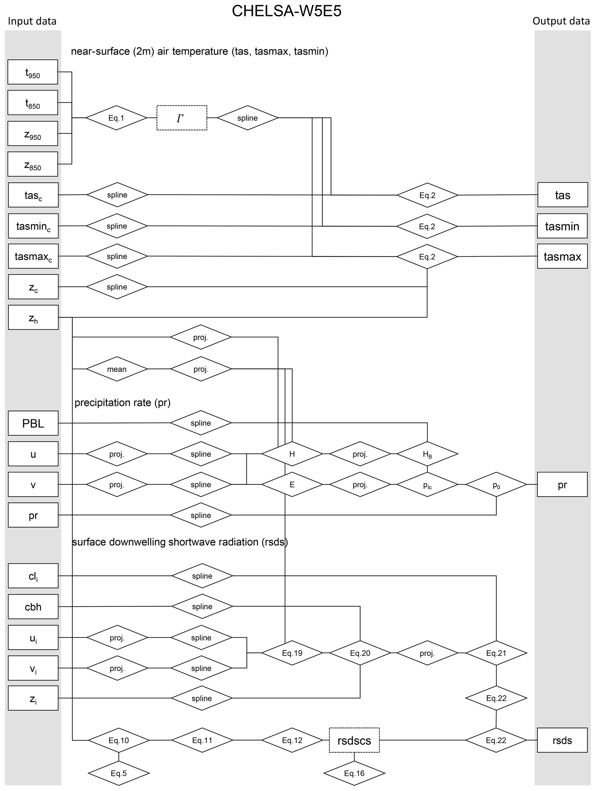 Figure 1 | Schematic representation of the most important calculation steps (rhombi) and input and output data (rectangles) of the CHELSA V.2.1 downscaling from (https://doi.org/10.5194/essd-15-2445-2023). Intermediate data icludes temperature lapse rate; and clear-sky solar radiation; rsdscs). Only the most important equations are indicated. Spline indicates that a B-spline interpolation is used to change the spatial resolution to a higher target resolution. Mean indicates that the mean across grid cells is used. Proj. indicates that a reprojection to another geographic projection is performed. For the respective abbreviations, see the equations in the main text.
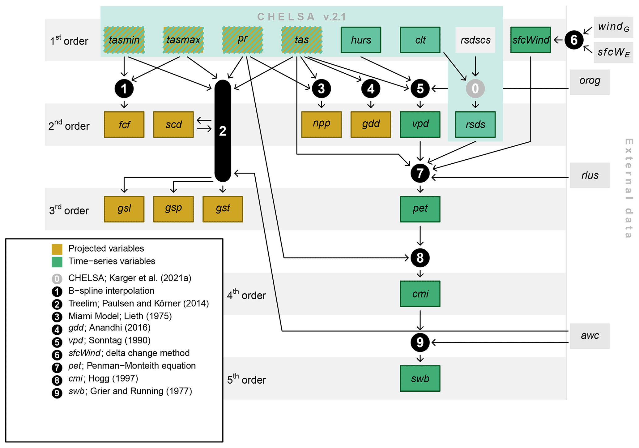 Figure 2 | Input data, analyses, and output variables generated in the BIOCLIM+ dataset based on CHELSA V2.1. tasmin represents daily minimum near-surface air temperature; tasmax represents daily maximum near-surface air temperature; pr represents precipitation rates; tas represents near-surface daily average air temperature; hurs represents near-surface relative humidity; clt represents cloud area fraction; rsdscs represents surface downwelling shortwave radiation assuming clear sky; orog represents orography; fcf represents frost change frequency; scd represents snow cover days; npp represents potential net primary productivity; gdd represents growing degree days; vpd represents vapor pressure deficit; rsds represents surface downwelling shortwave radiation corrected for atmospheric transmissivity and topography; sfcWind represents near-surface wind speed; sfcWE represents near-surface wind speed from ERA5; windG represents wind speed from the Global Wind Atlas; rlus represents surface upwelling longwave radiation; gsl represents growing season length; gsp represents growing season precipitation; gst represents growing season temperature; pet represents potential evapotranspiration; cmi represents the climate moisture index; awc represents available soil water capacity; swb represents site water balance. Green squares represent climate variables for which monthly time series are available for the period 1980–2018; orange squares represent variables for which future projections of climatologies exist; hashed squares represent variables with both time series for the recent past and future projections. Squares with border lines are part of the dataset presented.
Input Data:
CHELSA V2.1 downscales gridded climate fields from global reanalysis or Earth system model outputs, which provide coarse-resolution atmospheric variables. The input data include daily fields of air temperature (ta), near-surface air temperature (tas, tasmax, tasmin), wind components (ua, va, uas, vas), relative humidity (hur, hurs), precipitation flux (pr), surface air pressure (ps), cloud area fraction (cl, clt), geopotential height (zg), downwelling shortwave and longwave radiation (rsds, rlds), and near-surface wind speed (sfcWind). Temperature fields are used both at the surface and through the vertical atmosphere to calculate atmospheric lapse rates. Wind components from surface and upper air levels are required to estimate windward and leeward terrain effects. Cloud and humidity profiles are combined with elevation to refine estimates of surface relative humidity and cloud cover. Geopotential height fields are necessary to vertically interpolate atmospheric variables. Orography data are based on the a high resolution digital elevation model, providing the terrain basis for the downscaling of all variables.
Downscaling Methodology:
The downscaling approach in CHELSA V2.1 is a terrain-based, mechanistic method that transforms coarse-resolution atmospheric data into fine-scale climate information by explicitly accounting for topographic influences. Rather than relying on statistical relationships, it uses physical principles and high-resolution terrain data to simulate how climate variables are modified by elevation, slope, aspect, and wind exposure. Coarse atmospheric fields are first interpolated using multilevel B-spline functions. These fields are then adjusted based on terrain-sensitive transfer functions. Temperature is corrected using dynamically calculated lapse rates derived from vertical air temperature profiles. Precipitation is redistributed according to orographic uplift and leeward drying, based on near-surface wind vectors and planetary boundary layer height. Shortwave radiation is modified by terrain shading and slope orientation. For relative humidity (hurs), downscaling considers the atmospheric lapse rates combinded with the windward and leeward sides of mountains. Cloud area fraction (clt) is adjusted using pressure-level cloud fields combined with windward-leeward indices to simulate enhanced cloud formation over rising terrain. Near-surface wind speed (sfcWind) is downscaled using a vertical B-spline interpolation through all pressure levels of the atmosphere. Surface pressure (ps) is recalculated at high resolution using hypsometric equations that relate pressure to elevation and temperature.
Bias correction:
Bias correction in CHELSA V2.1 is applied exclusively to precipitation. The correction uses the Global Precipitation Climatology Centre (GPCC) dataset, but only at grid cells that contain actual meteorological stations. At these locations, the bias is calculated as the ratio between the observed GPCC precipitation and the modelled precipitation from the downscaled field, on a monthly basis. As meteorological station can still observe a bias (gauge undercatch) specifically in snow dominated areas, we additinoally add the bias correction surface from Beck et. al. 2020 (https://doi.org/10.1175/JCLI-D-19-0332.1) at a 1km resolution. This bias surface is then interpolated using a multilevel B-spline method to produce a continuous correction grid. The interpolated monthly bias is finally applied to the daily downscaled precipitation fields, ensuring temporal consistency while preserving the spatial correction derived from observational data.
Validation summary:
The validation of CHELSA V2.1 focused on evaluating the accuracy gains from topographic downscaling for key climate variables including near-surface air temperature (tas, tasmax, tasmin), precipitation (pr), surface downwelling shortwave radiation (rsds), relative humidity (hurs), wind speed (sfcWind), and cloud area fraction (clt). The evaluation used station-based observational datasets, primarily GHCN-D for temperature and precipitation, and GEBA for radiation. Across all variables, the downscaling procedure significantly improved spatial detail and reduced systematic biases, particularly in topographically complex regions. Compared to the coarse-resolution W5E5 forcing data, downscaled CHELSA data consistently showed: Higher correlations with station observations (typically r > 0.9), Reduced bias, especially for temperature and precipitation, Lower root mean squared errors (RMSE) and mean absolute errors (MAE). Air temperature (tas, tasmax, tasmin): Topographic lapse-rate-based downscaling led to strong improvements in complex terrain, with bias reductions and improved correlation. However, for tasmin, the downscaling occasionally introduced bias in cold-air pooling regions due to the limitations of using mean daily lapse rates for nocturnal inversions. Precipitation (pr): The largest performance gains were observed in mountainous regions, where orographic effects are strongest. Downscaling preserved the spatial variability and improved local accuracy. However, the method cannot capture convective precipitation, which limits performance in flat regions during extreme events. Shortwave radiation (rsds): Biases were substantially reduced through terrain-informed clear-sky radiation modeling and cloud corrections. However, correlations were slightly reduced at high values of rsds, likely due to over-simplified atmospheric transmissivity assumptions. Relative humidity (hurs) and cloud area fraction (clt): These variables showed high spatial coherence with atmospheric dynamics and topography. Monthly climatologies of clt correlated well with observational data (r = 0.84), even without explicit treatment of convective clouds. Wind speed (sfcWind): Validation showed good agreement with observed distributions. Bias correction using the Global Wind Atlas and ERA5 reanalysis improved local accuracy, especially in wind-exposed terrain. Comparison with Dynamically Downscaled Data: When benchmarked against the Weather Research and Forecasting (WRF) model over North America, CHELSA’s downscaled air temperature and precipitation performed similarly or better, particularly in terms of bias reduction and correlation with observations.
Variable specific downscaling algorithms:
Depending on the variable, different downscaling algorithms are applied:
| variable | Downscaling |
| tas, tasmax, tasmin | Temperature is downscaled based on the relationship between elevation and atmospheric temperature. In general, air cools with increasing altitude — a pattern described by the lapse rate. The model first interpolates coarse temperature fields to a finer grid and then adjusts these values according to the local topography. Where terrain is higher than the surrounding area, temperatures are reduced; where it is lower, they are increased. This lapse rate adjustment captures fine-scale variations in temperature caused by mountains, valleys, and slopes. The same principle is applied to daily mean, maximum, and minimum temperatures. While this method works well in most landscapes, it can be less accurate in conditions like nighttime cold-air pooling, where local temperature patterns deviate from the general lapse rate. Still, it substantially improves temperature representation in complex terrain compared to uncorrected coarse-resolution data. |
| rsds | Shortwave solar radiation is downscaled by simulating how sunlight interacts with topography and atmospheric conditions. The process begins by calculating the amount of incoming solar radiation under clear-sky conditions, based purely on solar geometry (sun angle, time of year, latitude) and the shape of the terrain. This includes how much a location is exposed to the sky (sky-view factor), the slope and aspect of the surface, and whether it is shaded by surrounding terrain at different times of day. Once this clear-sky radiation is estimated, the model adjusts it using cloud cover information. Clouds reduce the amount of solar energy that reaches the surface. The model incorporates the effects of total cloud area fraction (clt), accounting for how cloudiness varies with topography and wind direction, to more realistically simulate the reduction in solar radiation reaching the ground. This approach allows the model to distinguish between sun-exposed and shaded areas and between clear and cloudy conditions. By combining topographic effects with atmospheric cloud cover, the resulting radiation estimates provide high spatial detail and improved realism, especially in mountainous or highly variable landscapes. |
| clt | Cloud area fraction describes the proportion of the sky covered by clouds as seen from the ground. The downscaling approach simulates how terrain influences cloud layering and visibility using vertical profiles of cloud fractions and geopotential height across the atmosphere. The key principle is that clouds form and behave differently across elevation gradients and terrain exposure. The model first collects cloud fraction values at multiple atmospheric heights, and interpolates these values vertically to simulate a continuous cloud cover profile from the surface upward. This gives a fine-scale vertical “stack” of cloud coverage above each location. To determine which parts of the profile count as cloud-covered, the model applies a minimum cloud cover threshold, and identifies “cloud blocks” — contiguous vertical sections that exceed this threshold. Next, topography and wind effects are used to adjust the visibility and influence of these cloud blocks. For instance: Cloud layers closer to the surface are weighted more strongly, especially when the location is wind-exposed, as uplift supports condensation and cloud formation. In leeward or shielded areas, or where the terrain is located below the cloud base height, cloud influence is reduced. Finally, the model uses the maximum-random overlap assumption — a common method in atmospheric modeling — to combine individual cloud blocks into a single cloud area fraction at the surface. This means overlapping clouds in height are treated partly as stacked (maximum overlap) and partly as randomly layered (random overlap), reflecting realistic cloud layering. This approach provides a spatially and vertically nuanced estimation of surface-level cloudiness, influenced by both the 3D structure of clouds and the terrain. |
| hurs | Relative humidity near the surface reflects how much moisture is present in the air compared to the maximum it could hold at a given temperature. Accurately representing this variable is essential for understanding fog formation, evapotranspiration, and plant stress. The downscaling of hurs starts by using relative humidity values across atmospheric pressure levels, which are interpolated horizontally to the target high-resolution grid. Then, for each high-resolution pixel, a vertical interpolation is performed to estimate the humidity at the local surface elevation — rather than at a generalized coarse elevation — accounting for topographic variation. However, surface humidity is not only a function of elevation. To capture terrain-driven asymmetries, the model integrates a windward-leeward correction: On windward slopes, where moist air ascends, relative humidity increases due to cooling and potential condensation. On leeward slopes, where air descends and warms, relative humidity decreases. This correction is applied using a wind exposure index (calculated from wind direction and terrain structure), which enhances or reduces the interpolated surface humidity accordingly. In doing so, the model simulates terrain-induced microclimatic differences — for example, moist fog-prone forests on one side of a mountain, and drier zones on the other. |
| ps | Surface pressure in CHELSA is downscaled by adjusting coarse-resolution pressure values based on the elevation of each fine-scale grid cell. This adjustment follows the physical principle that air pressure decreases with altitude and that the rate of this decrease depends on both temperature and the lapse rate, which is the rate at which temperature changes with altitude. The process uses coarse-resolution surface pressure and temperature values and corrects them for the difference between the coarse grid elevation and the actual high-resolution terrain elevation. The adjustment takes into account the local temperature, since colder air leads to a steeper pressure drop, and the lapse rate, which modifies the pressure gradient depending on how quickly temperature declines with height. As a result, surface pressure is recalculated for each high-resolution location to reflect the realistic influence of topography, ensuring that pressure decreases appropriately in mountainous areas and remains higher in lowlands. |
| sfcWind | Surface wind speed is calculated by interpolating atmospheric wind components from multiple vertical levels down to the elevation of the terrain surface. Specifically, the model begins with u (east-west) and v (north-south) wind components defined at several pressure levels in the atmosphere. These components are vertically interpolated to the surface using geopotential height and high-resolution terrain elevation. Once interpolated to the surface height at each fine-scale grid cell, the u and v components are converted from Cartesian to polar coordinates to derive wind direction and magnitude. The final surface wind speed (sfcWind) is represented by the magnitude of this vector. |
| tz | The temperature lapse rate (tz) represents the rate at which air temperature decreases with elevation. It is calculated daily from vertical temperature profiles in the lower atmosphere. Specifically, temperature differences between two atmospheric levels are used to estimate the lapse rate at each time step. This rate is then applied to correct coarse-resolution temperature data according to the local elevation from a high-resolution digital elevation model. The result is a spatially refined representation of near-surface temperature that reflects topographic variation. |
| pr | Precipitation is downscaled by simulating key orographic processes: Wind Effect: The model calculates a wind exposure index for each grid cell using wind components. Terrain is scanned in the wind direction to assess whether a location is windward (more exposed, more rain) or leeward (sheltered, less rain). This is done using a directional terrain scan based on slope and relative elevation. Boundary Layer Correction: Terrain influence is strongest where the surface intersects the planetary boundary layer (pbl), the lowest part of the atmosphere where most weather occurs. CHELSA V2.1 uses pbl heights to adjust the wind effect based on how much the terrain penetrates this layer, reducing unrealistic orographic influence where terrain is either too low or too high. Valley Exposition: High mountain valleys can be rain-shadowed even when nearby peaks receive substantial precipitation. CHELSA V2.1. includes a valley exposition index that simulates how deeply embedded a valley is and reduces precipitation accordingly. These mechanisms are used to redistribute the total precipitation within each coarse grid cell, scaling the values to match the original coarse grid totals while resolving realistic local variability. Compared to CHELSA V.1.2 the wind effect and valley exposition effect has been calculated at a horizontal resolution of 3km instead of 1km to correct for the too strong orographic effects in V.1.2. |